The Moneyball of Real Estate: Ames housing price prediction

This post walks through my Ames housing price prediction project, where I built and deployed a machine learning ensemble to estimate sale prices.

I. Introduction

The Flipper’s Dilemma In real estate, the line between a “deal” and a “money pit” is often invisible. Most investors rely on gut feel or “back-of-the-napkin” math to estimate a renovation’s return on investment (ROI). “If I add a garage, this house will surely sell for $30k more, right?”

I wondered: What if I didn’t have to guess? How could I be assured that the improvement I make to the home will increase its sale value by the amount I spent or more? My goal was to move beyond the standard Kaggle-style objective of simply predicting a price. I wanted to build a Decision Support System an end-to-end machine learning pipeline that not only predicts fair market value but mathematically identifies the highest-ROI renovation opportunities in Ames, Iowa. Using a tech stack of Python, Scikit-Learn, XGBoost, CatBoost, and Shiny, I turned a static dataset into a dynamic investment engine. 

II. Data Engineering

The “None” Strategy Real-world data is messy, and the Ames dataset was no exception. Faced with over 80 columns of mixed quality data points, my first task was defining an imputation strategy that was robust enough for production.

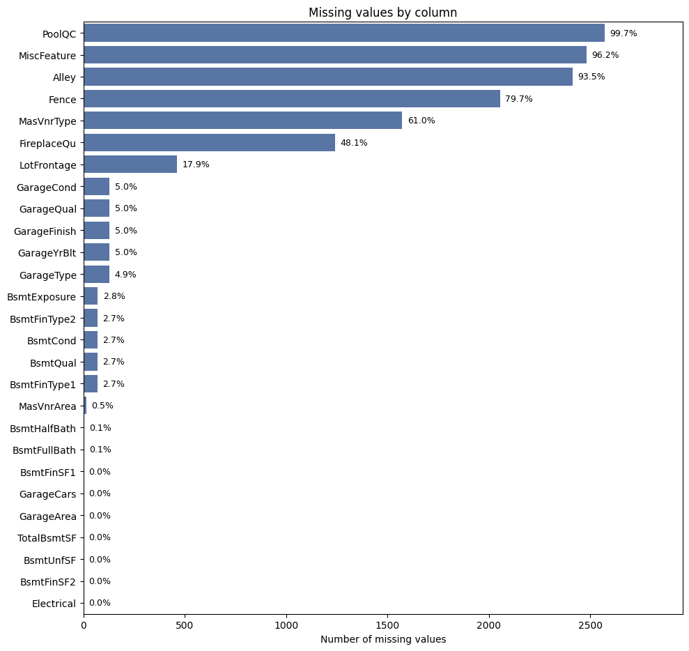
The dataset documentation suggested a manual approach -mapping specific NaN values to specific meanings (e.g., assuming a missing Pool Quality score meant “No Pool”). However, I decided to deviate from these manual rules to build a more generalized pipeline. Hard-coding specific assumptions for 80+ columns creates ‘technical brittleness’-a system prone to breaking if data schemas shift. I wanted a scalable architecture that applied consistent logic across the board, reducing the risk of human error and making the pipeline easier to maintain in production. 

• The Strategy: Instead of manually hard-coding definitions for every column, I adopted a systematic imputation strategy.
  • Categorical Data: I filled all missing values with the string “None”. This treated “missingness” as its own distinct category, allowing the model to learn the signal behind the absence of data without me imposing assumptions.
  • Numerical Data: I imputed missing values with the Median.

This decision paid off. Letting the model interpret the “None” category resulted in it learning that missing values in key columns like BsmtExposure were strong signals of lower value. While the data dictionary instructs us to manually map these NaNs to “No Basement,” my approach allowed the model to mathematically validate this relationship independently-effectively capturing the “lack of feature” penalty without requiring complex manual mapping scripts.

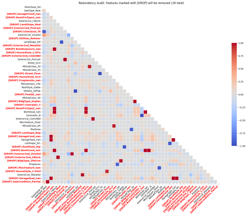
To ensure the model remained lean, I performed a “Redundancy Audit.” Using a Correlation Threshold, I identified features that were essentially saying the same thing, By cutting the fat and removing multicollinear variables, I reduced the risk of overfitting and ensured that each coefficient in my final model had a clear, independent meaning.

III. The Model Battle Royale

Glass Box vs. Black Box I approached modeling as a competition between two philosophies: the interpretable “Glass Box” and the high-performance “Black Box.”

Phase 1: The Glass Box (Linear Models)

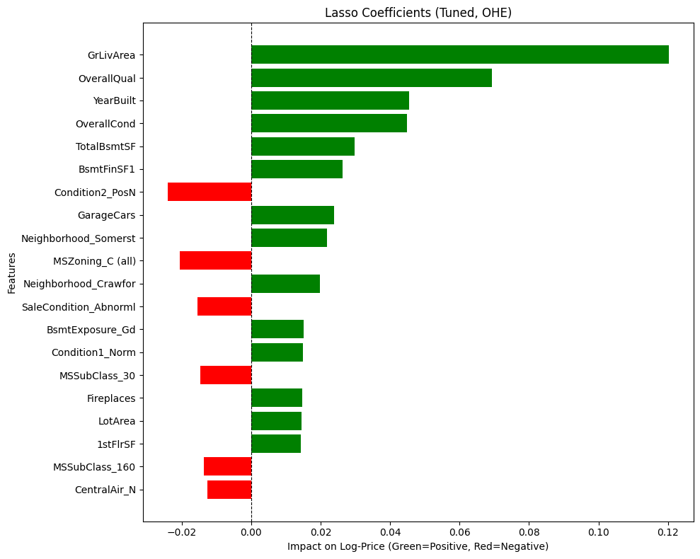
I started with OLS, Lasso, Ridge, and ElasticNet. These models are the “strict accountants” of machine learning. They are highly interpretable, allowing me to see exactly how many dollars a fireplace adds to the price tag. But they struggle with nuance.

• The Finding: While ElasticNet tried to be the “pragmatist” by taming the Living Area coefficient (reducing it from Lasso’s >0.12 to ~0.10), Lasso emerged as the clear winner, achieving the highest mean Cross-Validation R2 (0.8899) of all the linear models. Lasso proved to be “Size Obsessed,” assigning massive value to Ground Living Area, but it also provided the most sensible prioritization of the fundamentals: Overall Quality (fit and finish), Overall Condition (maintenance), and Year Built (age). It effectively zeroed out “noise” like Pool Area, telling me: “Ignore the fluff. The safest way to add value is to maintain the property and make it bigger.”

• The Lesson: Trust the coefficients, not just the score. My OLS baseline produced a competitive R2, but inspecting the coefficients revealed it was “fitting the noise.” Due to multicollinearity, OLS made illogical trade-offs. For example, it assigned a positive value to YearBuilt but a negative penalty to SaleType_New, despite these features describing the same “newness.” 
  
  Regularization (Lasso/Ridge) didn’t just tune the model; it acted as a “Logic Filter,” dampening these contradictions to ensure the model’s advice was not just statistically accurate, but practically sound.

Phase 2: The Black Box (Tree Models & SVR)

Next, I moved to the non-linear powerhouses: SVR, Random Forest, XGBoost, and CatBoost. This wasn’t just about trying different algorithms; it was about finding the right architectural fit.

• The Honorable Mentions (SVR & Random Forest):
  • SVR (Linear Kernel): While stable and reliable in its feature attributions, SVR hit a performance ceiling with a CV score of ~0.87. It simply lacked the capacity to capture the complex, non-linear interactions required to break the 0.90 barrier.
  • Random Forest: This model revealed a fatal flaw I call “The Monolith.” It assigned a staggering 55% feature importance to a single variable-Overall Qual. This made the model unbalanced and dangerously sensitive to a subjective rating, failing to capture the nuance of the rest of the dataset.
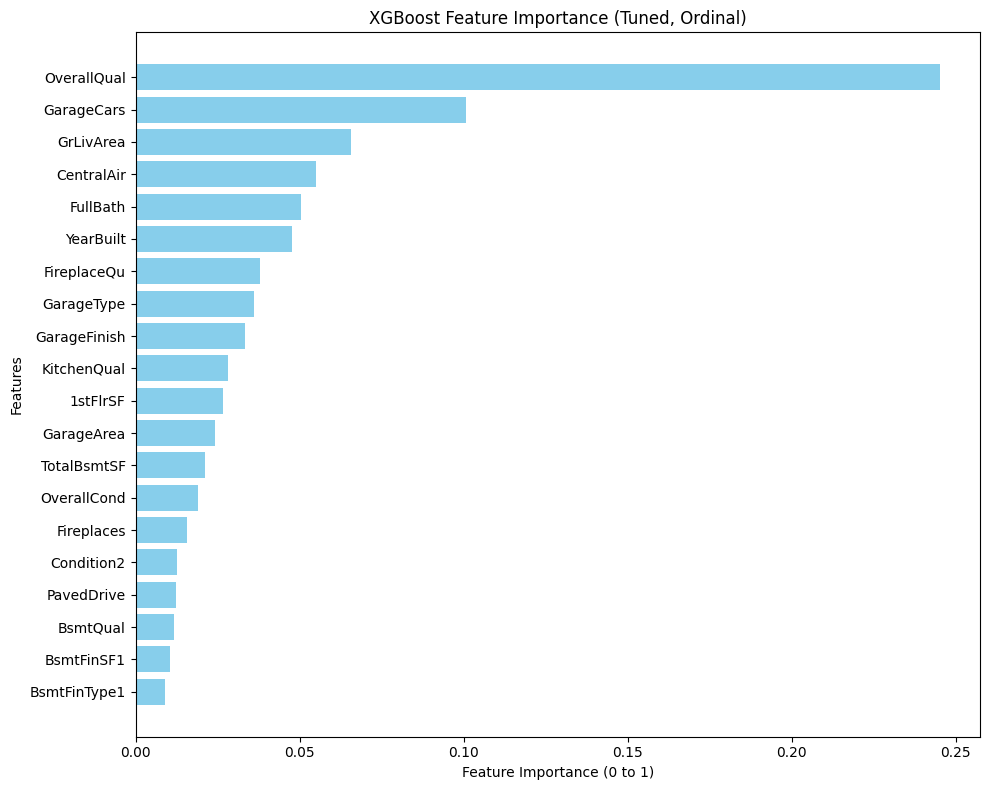
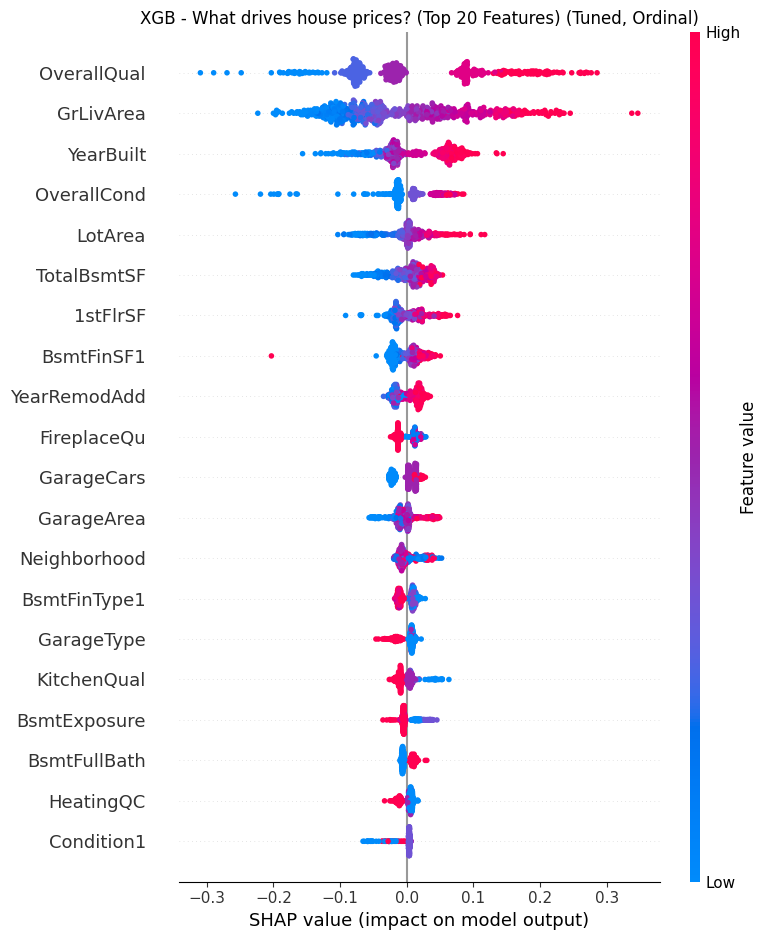
• The Champions (XGBoost & CatBoost): The Gradient Boosters changed the game, with both models exceeding 0.91 CV scores-the highest of any individual models tested.
  • The Finding: Unlike Random Forest, they offered a balanced worldview. XGBoost emerged as the “Amenities Flipper,” ranking GarageCars as a top driver (even higher than living area), proving that premium features can outweigh raw square footage.

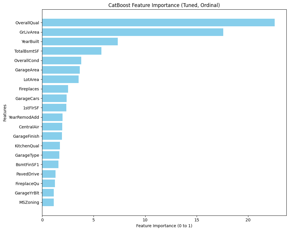
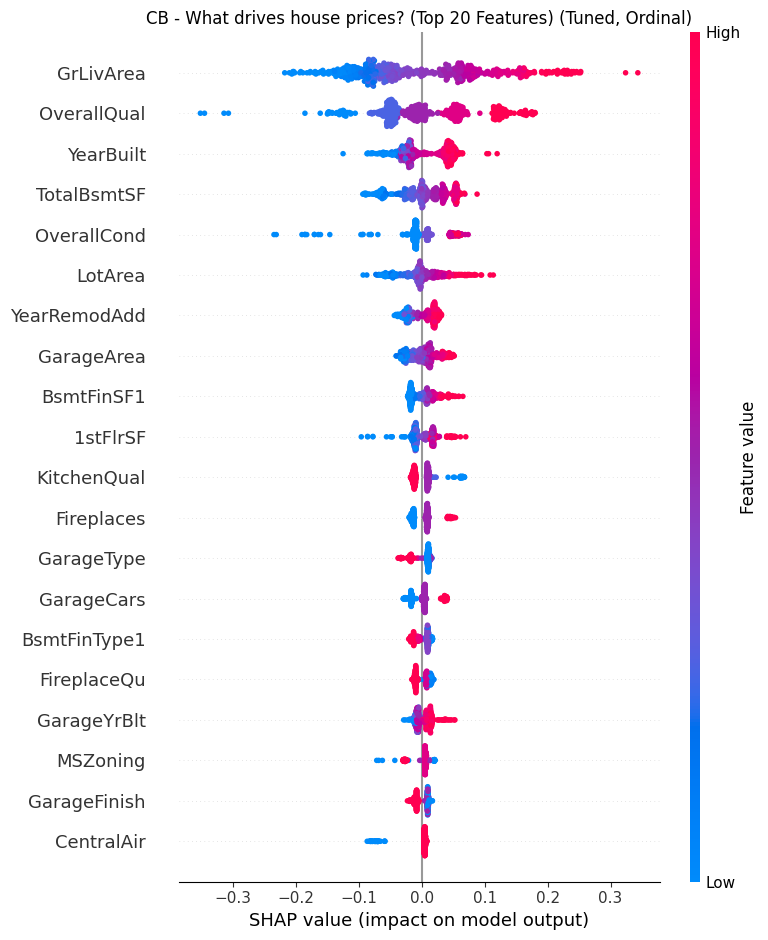
• The Synergy: I selected both for the final ensemble because they are strong learners that “think” differently. XGBoost grows asymmetrically (leaf-wise) to capture specific, deep interaction rules, while CatBoost grows symmetrically (oblivious trees) to act as a regularizer. This structural diversity meant they could cover each other’s blind spots rather than repeating the same errors.

• The Lesson: Don’t flatten the hierarchy. One-Hot Encoding destroys the natural order of real estate data (e.g., Excellent > Good > Poor), treating them as unrelated buckets. By switching to Ordinal Encoding, I preserved this mathematical rank, enabling the trees to make logical splits based on “Quality Thresholds” (e.g., Condition ≥7) rather than memorizing isolated features. This allowed the model to capture the “tipping points” where value accelerates.

Phase 3: The “Super Model” (Voting Regressor)

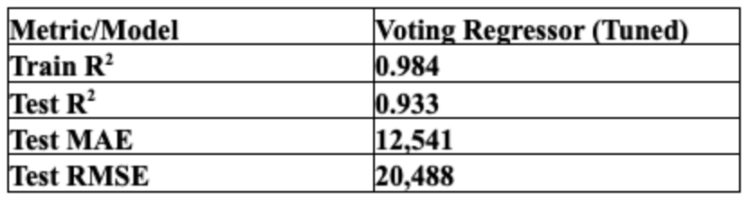
Why choose one worldview? I built a Voting Regressor that combines the disciplined baseline of Lasso (Weight: 1) with the aggressive precision of XGBoost and CatBoost (Weight: 2 each).

• The Strategy: This hybrid architecture was designed to balance the “Square Footage” fundamentals (Lasso) with the “Luxury Amenity” premiums (Trees). The linear model provided a stable pricing floor, while the boosters captured the non-linear value ceilings that simple math missed. 
• The Pipeline Feat: The real engineering challenge was data routing. I built a custom pipeline that simultaneously fed One-Hot Encoded data to the Lasso branch and Ordinal Encoded data to the Tree branches. This ensured every model received the data in its optimal format-preventing the “dilution” of the trees while satisfying the “math” of the linear model-ultimately driving the ensemble to a Test R2 of 0.933.

IV. Productionizing

From Lab to Factory A model in a notebook is a prototype; a model in an app is a product. The transition required solving the “Well, it works on my machine” problem. To productionize the Ames housing price prediction pipeline, I packaged preprocessing and inference behind a Flask REST API and a Shiny for Python dashboard.

• The Unified Pipeline: I wrapped my entire preprocessing, imputation, and modeling logic into a single Scikit-Learn Pipeline. This means raw user input-JSON data-goes in, and a prediction comes out, without any manual data prep. 
• Technical Spotlight: Custom Feature Engineering: Tο ensure the pipeline was robust and portable, I built custom classes-Feature Engineer and Correlation Threshold-that inherit directly from Scikit-Learn’s BaseEstimator and TransformerMixin. This architecture allowed me to bake complex logic directly into the pipeline object: 
  • Automated Engineering: My Feature Engineer class standardizes the creation of high-signal features like TotalSqFt, HouseAge, and TotalBath.
  • Geospatial Intelligence: If specific neighborhood data is provided, the class leverages the geopy package to fetch precise Latitude and Longitude coordinates, capturing micro-location value that simple labels might miss.
• Artifact Management: I didn’t just pickle the model. I created a synchronized “Artifact Factory” that exports ames_model_defaults.pkl (to auto-fill missing user inputs) and ames_model_options.pkl (to populate the dashboard’s dropdowns dynamically). 
• The Testing Suite: I built a three-tier testing framework to ensure reliability:
  • The Mega-Mansion Test (Safety): I fed the API a 200,000 sq ft house. Instead of crashing or predicting $500 Million, my tree-clamping logic kept the prediction grounded.
  • The Ghost House (Stability): I tested inputs with 0 sq ft to ensure the model threw appropriate errors rather than nonsensical prices.

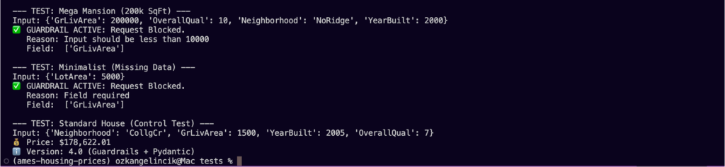
• The Renovation Check (Logic): I wrote scripts to verify that Price(Renovated) > Price(Base). If adding a garage didn’t increase the price estimate, the model failed the logic test.

V. The “House Flipper Pro” Dashboard (Shiny)

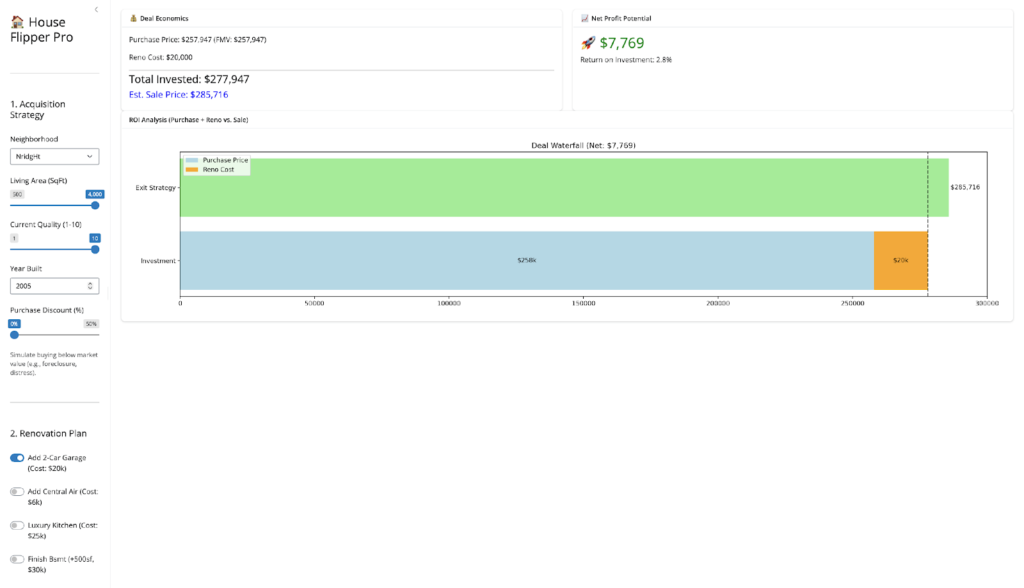
Finally, I visualized my engine using Python Shiny. I didn’t want a static report; I wanted a Deal Simulator. 

Try the Live App Here: House Flipper Pro

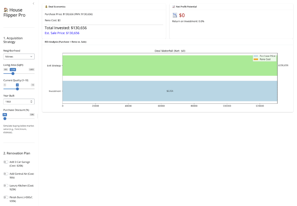
• The Control Center: I built an interface that lets me tweak every variable-Neighborhood, Quality, Square Footage to hunt for “Unicorn” deals in real-time.
• The Renovation Toggles: I added one-click buttons to simulate specific upgrades (e.g., “Add Central Air,” “Finish Basement”). This allows me to instantly see if a $20k garage adds $20k in value (Spoiler: usually not).
• The Deal Logic: I included a “Purchase Discount” slider and a dynamic Waterfall Chart. This enforces the discipline of the model: showing visually that true profitability usually comes from the buy, not just the fix.

VI. Strategic Takeaways: The Renovation Reality

The most exciting part of this project wasn’t the code; it was the real estate strategy the model revealed. 

• The “AC Arbitrage”: My model identified a consistent arbitrage opportunity in “Old Town.” Older homes there are heavily penalized for lacking Central Air. But I discovered a hidden multiplier: Square Footage. The data reveals that the market punishes the lack of central air far more severely in large homes than in small ones, creating a non-linear opportunity for value creation. 
  • The “Unicorn”: A large (2,500+ sq ft), Pre-1960s home without AC is the most profitable renovation target in the dataset. The market punishes these “obsolete” giants severely, so bringing them up to modern standards creates an outsized value lift compared to the fixed renovation cost.

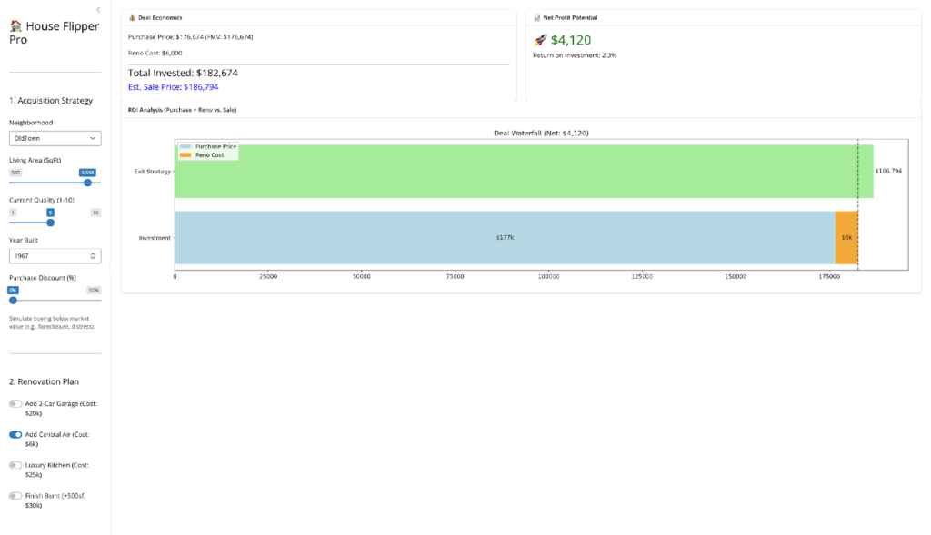
• The Garage Trap (vs. The Quality Leap): Conversely, the model warned me against adding garages without doing the math first. While many flippers assume a garage is a guaranteed “value-add,” the data tells a more complicated story.
  • The Findings: As the simulation above shows, adding a 2-car garage in a top-tier neighborhood does increase value for larger, high-quality homes—generating a $7,769 profit (2.8% ROI) on a $20,000 investment. However, in lower-tier neighborhoods, this math often flips to a net loss. This surprise finding highlights the danger of “Over-Improvement.” Budget-conscious neighborhoods often have invisible price ceilings, meaning buyers simply cannot pay the premium for a brand-new garage, causing the fixed cost of construction to exceed the value added.
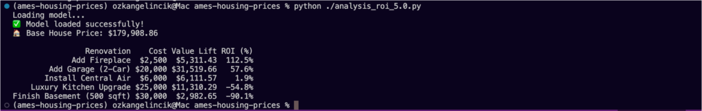
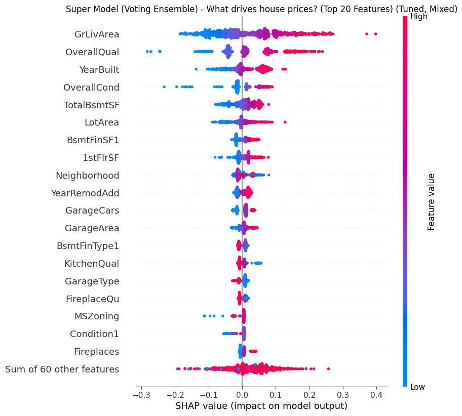
  • The Better Play: My “Super Model” (see SHAP summary below) revealed that Overall Quality is often a stronger, safer driver than amenities. Instead of risking $20k on a garage for a 2.8% return, the data suggests a higher and safer ROI comes from cosmetic upgrades (flooring, paint, fixtures) that bump a house from “Average” to “Good” condition—capitalizing on the model’s heavy weighting of the OverallQual feature.

VII. Future Roadmap

While the application is currently live and stable, the engineering journey continues. The next major step is Dockerization-containerizing the application to ensure it runs identically in any environment, eliminating the remaining “system dependency” risks and making the deployment truly cloud-agnostic.

VIII. Conclusion

The Golden Rule: Perhaps the most humbling finding from my Shiny app was this: Renovations rarely pay for themselves if you pay full price for the house. The “Purchase Discount” slider suggested that the best ROI doesn’t come from granite countertops; it comes from finding properties that are underpriced to begin with. My model confirms the old real estate adage: You make your money when you buy, not when you sell.

By combining rigorous data engineering with a “Super Model” ensemble, I turned a static housing dataset into a dynamic tool for finding value. I didn’t just predict prices; I decoded the market’s behavior, proving that with the right data, you really can “Moneyball” real estate. 

Launch the App